Key Ideas

Note

For more details around the discussion here, please refer to our paper.

This a brief overview of the relevant terminology and the algorithm. The former is important to understand the documentation (if you’re in a hurry this is the section to cover), and the latter, to reason about why specific results are produced.

Terminology

• complexity or size: This is how you quantify the learning capacity of a model. Pretty much any quantity that helps a model learn better by reducing its bias, is a valid notion of complexity. Some common examples of this quantity are:

  • the depth of a Decision Tree

  • the depths of the individual trees or the number of trees in a Random Forest.

  • number of non-zero terms in a linear model

  • complexity may be a vector, e.g., the combination (max_depth, num_trees) for a Random Forest.

  The term complexity for size comes from the interpretability literature (as examples, see here and here).

• complexity parameter: this is different from complexity. While we may be interested in a certain notion of complexity, a training algorithm might not directly allow us to specify it - we often control it via a different parameter, which we refer to as the complexity parameter. Some examples of this are:

  • we might be interested in the depth of a Decision Tree, but most libraries allow us to control the max_depth. Here, the depth is the complexity, and max_depth is the complexity parameter.

  • for linear models, we may be interested in the number of non-zero terms (complexity), but most libraries allow us to control the L1 regularization coefficient (complexity parameter).

  It is typical for the complexity parameter to depend on the implementation. For ex, Decision Trees in scikit allow you to specify a max_depth, but C5.0 doesn’t. Logistic Regression in scikit doesn’t allow you to directly specify the number of terms with non-zero coefficients, but the R package glmnet does.

• unbounded model: This is the model you would normally learn. For ex., if you use cross-validation to train a decision tree on dataset, without fixing the max_depth, I refer to this as learning an unbounded model. If the depth that gives the highest generalization accuracy is depth=30, then 30 is the unbounded model complexity.

Algorithm

At a high level the algorithm is fairly simple:

• we first learn an oracle model, say a Random Forest, on the provided dataset

• the oracle assigns uncertainty scores to all training data instances

• we determine a distribution over these uncertainty scores - according to which instances are sampled to train the model of our choice, say a Decision Tree, for a given complexity, say depth=5.

Determining this optimal distribution is performed using an optimizer:

• The optimizer is run for evals number of iterations, where evals is provided by the user. For ex, in our original experiments, we had set evals=1000 or greater.

• In each iteration, a model with the given complexity is fit a few times (decided by a variable called sampling_trials; by default sampling_trials=3). This is to reduce variance.

• When done, the distribution that led to the most accurate model on a validation set is reported.

Today, the distribution used is an infinite mixture model of Betas and the optimizer is a Bayesian optimizer.

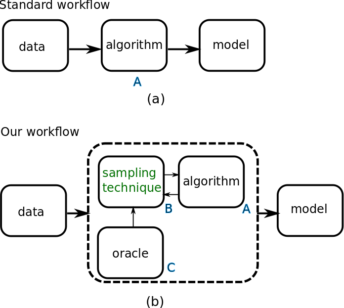
The following figure shows how the model training workflow changes:

1. this is how we normally train a model: a dataset is passed on to a training algorithm A, which produces a model.

2. this is what happens here: the data is used to produce an oracle C, which supplies information - only once - to our sampling technique/optimizer B, and the optimizer iteratively interacts with A to produce the model.

Of course, there are many additional details that make this tick, but they are not particularly relevant to using this library.

What to Expect

We looked at some results in the Quickstart page, but now let’s look the process visually. Consider this figure. The objective is to train a CART Decision Tree of depth=5 on the 2D-dataset shown in (a).

Source

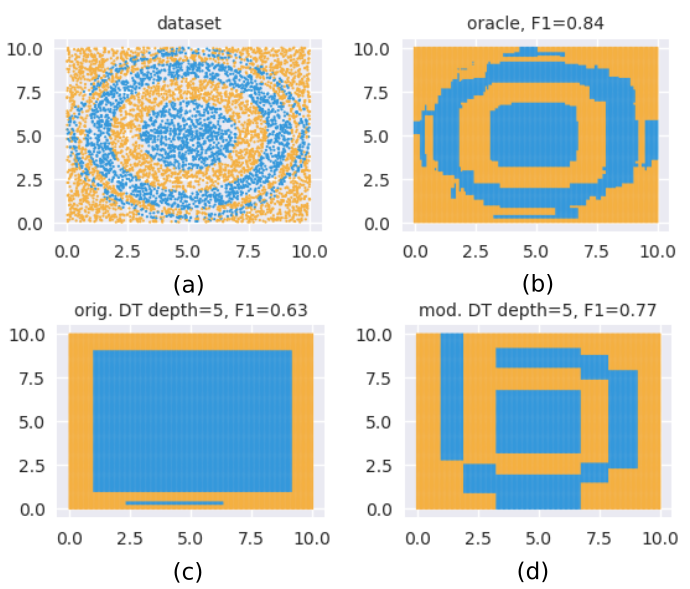
In (c), we see the boundaries such a tree learns; with a F1-macro=0.63, this is not great. (b) shows what our oracle learns, which here is a Gradient Boosted Decision Trees model; we see a much higher score of F1-macro=0.84, and also how the learned regions visually resemble (a). Our algorithm produces (d): also a CART Decision Tree of depth=5, but this time guided by the Gradient Boosted model. We see an improvement of 22% in the F1-macro score.

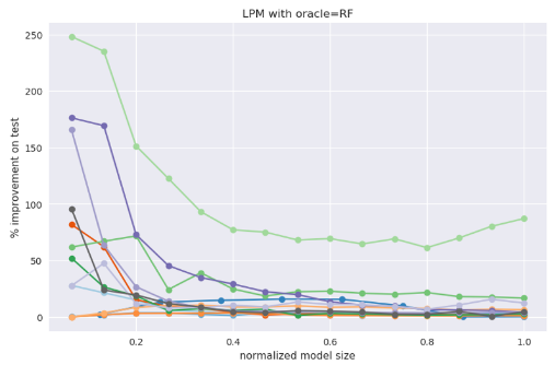
We have tried this on a bunch of datasets, and this small model effect - a small model can be positively influenced by a powerful oracle - shows up often. Here’s a plot of some of our experiments (source):

Here,

• different lines in the plot above denote different datasets - 13 in all.

• the plot is for training a Linear Probability Model (LPM) for different complexities; complexity here is the number of dimensions with non-zero coefficients in the LPM.

• the complexity range is normalized to lie within [0, 1] so that improvements for different datasets may be compared on the same plot

• the oracle used here is a Random Forest

• the typical pattern we observe is large improvements (sometimes 100%+!) are usually seen at small complexities, which fade away as model sizes increase

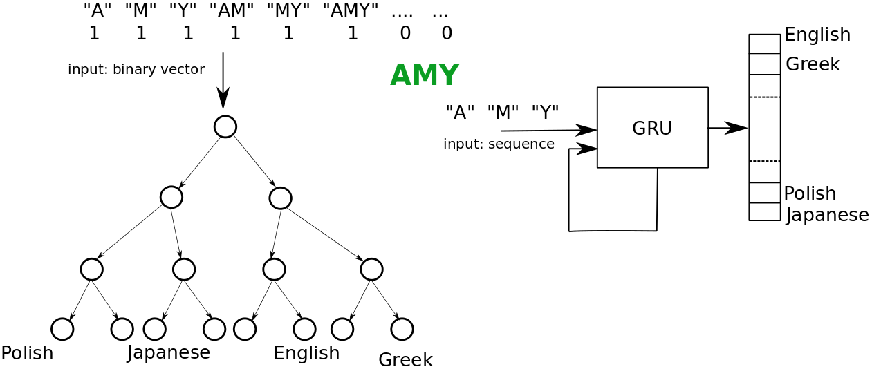
What is interesting is that this also seems to work across different feature spaces. For ex, our technique works in the following setup too:

• the objective is to predict nationalities based on names.

• the oracle is a Gated Recurrent Unit that processes a name one character at a time.

• the model of interest is a Decision Tree that uses character n-grams from the name.