Usage
Note
Remember to check out the Best Practices and FAQ too. Please Cite Us if you use the software.
The Essential API
The primary function to use is compactem.main.compact_using_oracle. While the docs cover the parameter details,
the semantics are described here. It’d help to read the Terminology and try out the
Quickstart example first.
A sample call might look like this:
from sklearn.datasets import load_digits
from compactem.oracles import get_calibrated_rf
from compactem.main import compact_using_oracle
from compactem.utils.data_format import DataInfo
from compactem.model_builder import GradientBoostingModel

X, y = load_digits(return_X_y=True)
d1 = DataInfo(dataset_name="digits", data=(X, y),
              complexity_params=[(2, 2), (2, 3), (4, 4)],
              evals=50)

# same dataset, but we will specify some fields as categorical
d2 = DataInfo(dataset_name="digits_with_categ_feat", data=(X, y),
              complexity_params=[(3, 3)],
              evals=100,
              additional_info={'categorical_idxs': [0, 1, 2]})

# we will use Random Forest as our oracle, but a reduced search space for this demo
results = compact_using_oracle(datasets_info=[d1, d2],
                               model_builder_class=GradientBoostingModel,
                               oracle=get_calibrated_rf,
                               oracle_params={'params_range': {'max_depth': [3, 5],
                                                               'n_estimators': [2, 5, 10, 30]}},
                               task_dir=r'output/usage_demo', runs=1)
Let’s understand what’s going on. In one call to compactem.main.compact_using_oracle, we may specify:
datasets, can be one or more : dataset(s) for which we want to build compact models. A dataset is always represented by the
compactem.utils.data_format.DataInfoobject, and multiple datasets need to be passed in as a list of such objects. This is the case here withdatasets_info=[d1, d2]. For each dataset, we may specify:one way to split the data into train, validation and test sets. This is optional, in which case there is default that is used. This is the case here.
one or more complexity parameters: denotes the complexity parameters for which we want to build models. This is dataset specific since for easily classifiable datasets you might not need a large range of parameters to explore.
In this example, for
d1we want to build models for the three complexity parameters[(2, 2), (2, 3), (4, 4)], while ford2we are just interested in one:[(3, 3)]. The parameters here are 2-tuples sinceGradientBoostingModelrequires bothmax_depthandnum_boosting_roundsas a parameter.number of optimizer iterations: denoted by the
evalsparameter. This is dataset dependent since for larger datasets or ones with a lot of classes, we might want a relatively lower number of iterations.additional info: model builders might accept additional information at initialization, which can be passed in via this parameter (expected to be a
dict). This is specific to the model builder. TheGradientBoostingModelcan be explicitly given the indices of the categorical features - which is what we the example shows with{'categorical_idxs': [0, 1, 2]}(the actual data is not categorical, but has integer values - this is only to illustrate usage).
model builder class, exactly one: this is denoted by
model_builder_class=GradientBoostingModelhere. I refer to such classes as model builders, since these are used to train the actual models we are interested in.oracle, exactly one: this is denoted by
oracle=get_calibrated_rf, whereget_calibrated_rf()learns a Random Forest classifier as an oracle, one each ford1andd2. This function will be passed in the additional parametersoracle_params, which decide the model selection search space (optional, since there are defaults available). These functions are referred to as oracle learners.task dir, exactly one: outputs from this function call - which are multiple files - are stored in this directory. This is
task_dir=r'output/usage_demo'in this example. The output files themselves need not be manually analyzed, since the function returns results as a dataframe, and for analysis in a subsequent session, it is recommended to use objects of the typecompactem.utils.output_processors.Result; these need to be instantiated with this output directory.
For other parameters and further details, see the docs at compactem.main.compact_using_oracle.
Outputs
The dataframe returned by compactem.main.compact_using_oracle has one row for each dataset and complexity (defined
for the dataset) combination. This is an “aggregate” result in the sense that individual runs are averaged over.
Each row has these fields:
dataset_name: name of dataset provided in the
DataInfoobjectcomplexity: the complexity of trained model
num_instances: total number of instances in the dataset
num_classes: number of classes
num_iterations: number of optimizer iterations
avg_original_score: mean of baseline scores i.e. w/o applying our algorithm, across runs for this complexity
std_original_score: std.dev. of original scores across runs for this complexity
avg_new_score: mean of new scores i.e. after applying our algorithm, across runs for this complexity
std_new_score: std.dev. of new scores across runs for this complexity
pct_improvement: percentage improvement of new over old score. Note: this calculated over the score averages, and is not the average of percentage improvements. This is done for robustness - since at smaller complexities, accuracy scores can be very small, they might lead to wildly different improvement values.
avg_oracle_score: mean oracle score - this does not change with complexity for a dataset; the averaging is over runs (the oracle is rebuilt per run)
std_oracle_score: std. dev. of the oracle score
avg_runtime_in_sec_total: mean wallclock runtime in seconds for this setting of complexity+run; includes building the baseline models, etc.
avg_runtime_in_sec_opt: mean wallclock runtime in seconds for just the optimization step
best_model_paths_json: this is where the optimal models are saved. This is a dict with the following stucture:
key: tuple of (baseline_score, new_score)
value: relative path of model file
There is one entry representing each run: the idea is users can pick a model that has the best baseline-to-new score model trade-off for them. NOTE that the path is not necessarily of the new model; it is for the best model: in cases where the percentage improvement is 0, this actually points to the baseline model.
Once compactem.main.compact_using_oracle has been run, these results can be accessed in a later session too,
since all of it is written into the task_dir. Instantiate a compactem.utils.output_processors.Result object,
with the same task_dir that was used in the original experimentation, and invoke the read_processed_results()
to access the results dataframe.
Some things to keep in mind:
The standard deviation is computed using pandas, which uses Bessel’s correction. So, if you only have one run, the std. dev. is not defined.
All scores are F1-macro scores; this is not configurable today.
The aggregate results match up the complexities of the baseline and new models. This might occasionally lead to unintuitive outputs. For ex, if we want to create decision trees of max_depth=5, it just might happen that the baseline and original trees end up with depths of 4 and 5 respectively. The output rows in the results dataframe compare baseline and new models for the same complexity of the new model, so baseline model numbers (for depth=4) would be absent.
The original raw results, including unmatched baseline scores, are not lost and are stored in intermediate dataframes - these can be obtained by setting the flag
all=Truein the call tocompactem.utils.output_processors.Result.read_processed_results.These are yet to be documented.
Namespaces vs Paths
You may have noticed that the filesystem paths don’t always align with the namespace. This is a deliberate decision to make import statements shorter. This is true in the following cases:
model builders: the actual path
compactem.model_builder.*.xyzis contracted tocompactem.model_builder.xyz. As an example, instead of importingcompactem.model_builder.DecisionTreeModelBuilder.DecisionTree, we importcompactem.model_builder.DecisionTree.oracle learners: the actual path
compactem.oracles.*.xyzis contracted tocompactem.oracles.xyz. An example iscompactem.oracles.oracle_learners.get_calibrated_rfis imported ascompactem.oracles.get_calibrated_rf.
The docstrings themselves point to the paths, and not to the namespaces.
Additional Stuff
Optimal Sample
There are some other interesting operations supported:
Since the core approach is to pick the best set of training instances, you can look at this final sample too. To do so:
remember to set the parameter
save_optimal_sample=Truein the call tocompactem.main.compact_using_oracle.Use the method
compactem.utils.output_processors.Result.get_optimal_sampleto fetch the optimal sample.
You can also control up to how many points from the original dataset might be used, using the
max_sample_sizeparameter in the call tocompactem.main.compact_using_oracle.
The following figure shows what an optimal sample might look like. The left-most image shows the dataset to be classified, and the two images on the right show the sample picked as well as the generalization area of Decision Trees of depths 1 and 4.
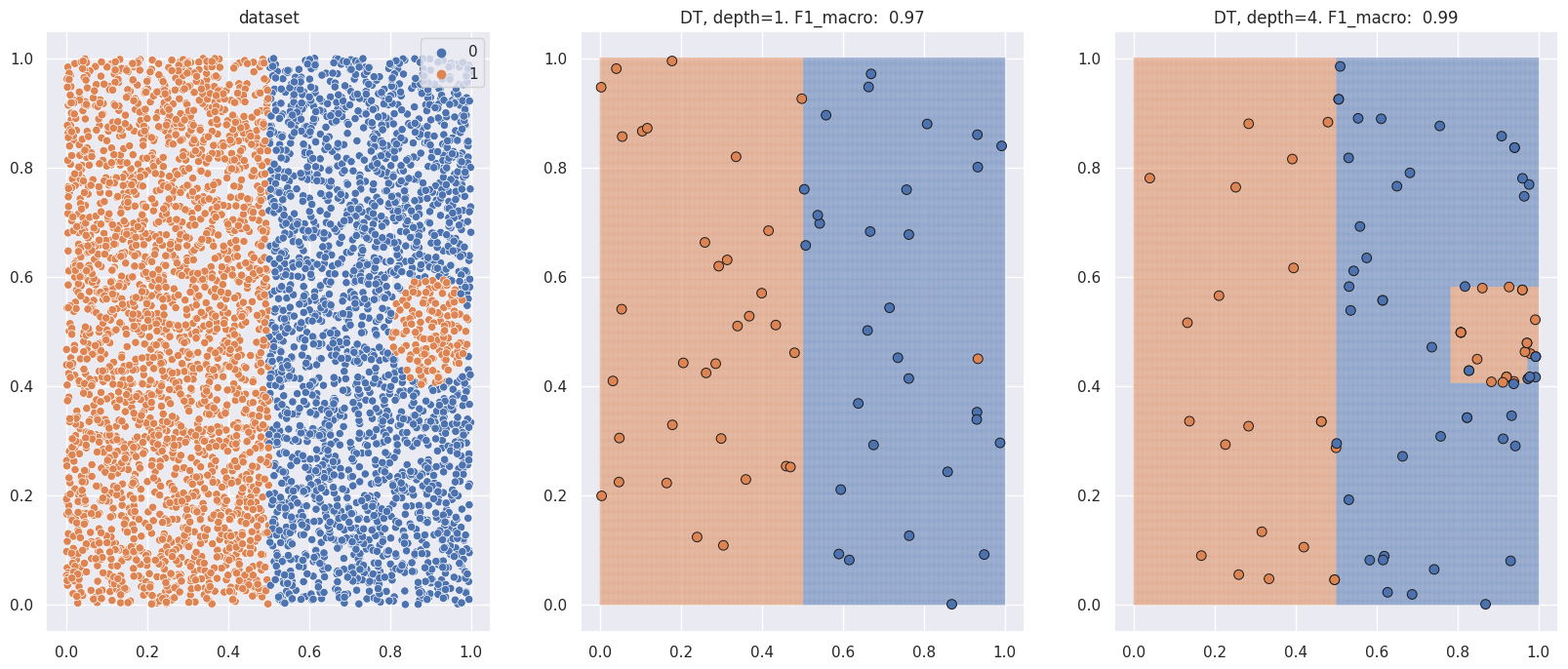
Note how in the first case, given the limited complexity, the tree ignores the small circular region. In the second case, it begins to sample there too.
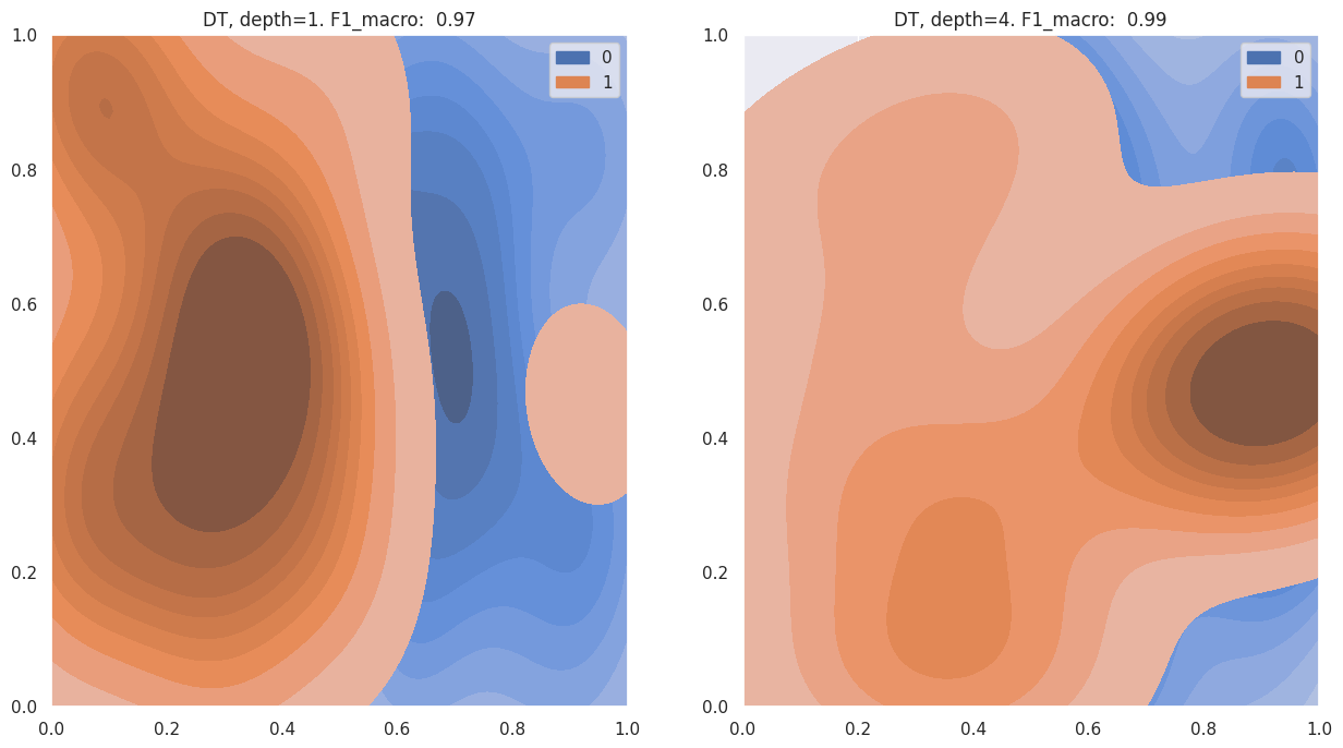
This is also visible in the KDE plots below - for the different depths (see titles). The second image has a more pronounced region for the positive label in and around the circle.
Caution
Interpreting the selected sample can be tricky. The optimizer might keep around certain points only because they were selected in the early random phase of the search, and they don’t influence accuracy to the extent they are later meaningfully retained or discarded.
Some combination of the model complexity and the maximum sample size might produce a meaningful subset, but I haven’t entirely explored this aspect.
Compaction Profile
One way to visualize the compaction obtained is by lining up the baseline complexities with the smallest complexity of among the new models that is at least as accurate as the baseline model. For ex, if we had constructed decision trees for max_depth values of 1…5 with this outcome:
complexity |
avg_original_score |
avg_new_score |
|---|---|---|
1 |
0.4 |
0.5 |
2 |
0.46 |
0.5 |
3 |
0.5 |
0.6 |
4 |
0.65 |
0.73 |
5 |
0.7 |
0.8 |
Then, the “compaction profile” i.e. the aligned complexities based on accuracies, would look like this:
baseline_complexity |
new_complexity |
|---|---|
1 |
1 |
2 |
1 |
3 |
1 |
4 |
4 |
5 |
4 |
This is effectively saying that a compact model of size 1 is as good as an original model of size 3, etc. This may be visualized in the following manner (source):
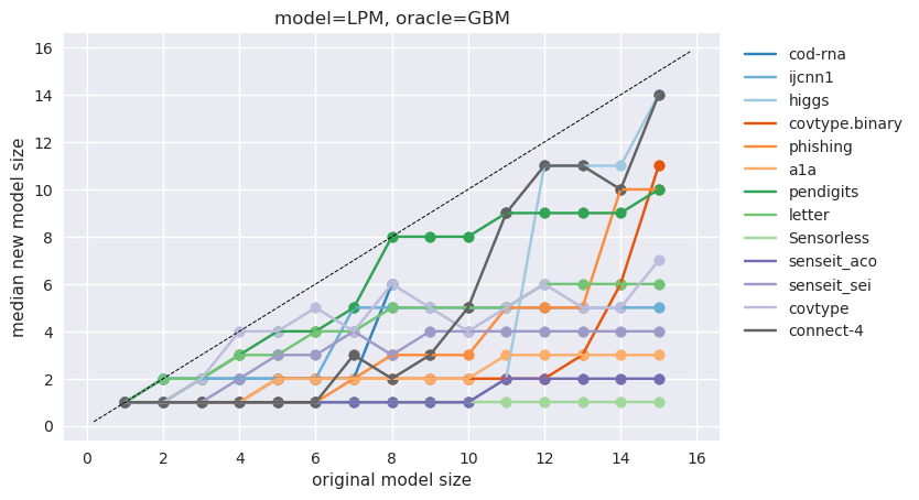
Here, every line represents a different dataset. This is for the combination of using a Gradient Boosted Model as an oracle for training Linear Probability Models.
The method compactem.utils.output_processors.Result.get_compaction_profile may be used to obtain this alignment.
No plotting utility is provided since the above plot makes sense only for scalar complexities.
Supported Models
Here’s a list of models currently supported.
oracle learners:
Random Forest - this is a wrapper over scikit’s Random Forest classifier.
Namespace:
compactem.oracles.get_calibrated_rf
Gradient Boosted Decision Trees - this is a wrapper over LightGBM’s gradient boosted decision trees.
Namespace:
compactem.oracles.get_calibrated_gbm
model builders:
Decision Tree - this is a wrapper over scikit’s Decision Tree classifier.
Namespace:
compactem.model_builder.DecisionTreeDoc:
compactem.model_builder.DecisionTreeModelBuilder.DecisionTreeComplexity Param: maximum depth of tree
Complexity: depth of tree
Linear Probability Model - uses scikit’s Least Angle Regression (LAR) implementation.
Namespace:
compactem.model_builder.LinearProbabilityModelDoc:
compactem.model_builder.LinearProbabilityModel.LinearProbabilityModelComplexity Param: number of features with non-zero coefficients. In case there are more than two classes, this is enforced per one-vs-all classifier.
Complexity: number of features with non-zero coefficients. In case there are more than two classes, this is enforced per one-vs-all classifier.
Random Forest - this is a wrapper over scikit’s Random Forest classifier.
Namespace:
compactem.model_builder.RandomForestDoc:
compactem.model_builder.RandomForestClassifier.RandomForestComplexity Param: max_depth, number of trees
Complexity: median depth of trees, number of trees
Gradient Boosted Decision Trees - this is a wrapper over LightGBM’s gradient boosted decision trees.
Namespace: compactem.model_builder.GradientBoostingModel
Doc:
compactem.model_builder.GradientBoostingClassifier.GradientBoostingModelComplexity Param: max_depth, number of boosting rounds
Complexity: max_depth, number of boosting rounds
Writing Custom Oracles and Models
As mentioned earlier, while the library supports certain model builders and oracle learners today, it is intended that a user is able to add their own models too. This is fairly easy.
oracle learners: lets start with oracles. If you want to use your own oracle, you have two options:
the simplest way is to not write one at all. Yep.
compactem.main.compact_using_oraclecan accept uncertainty values directly - check the docs. These are for cases like the oracle is in a different language, is a web service, or in general, time consuming to integrate.If you can procure the per-label model confidences, use the
compactem.core.oracle_transfer.uncertaintyfunction to convert them into uncertainties.the other way is to write a function that can accept a dataset (X, y) and learn an oracle model. If you are coming from scikit, note that this is different from the
fit()function: here you must generalize (via cross-validation et. al) and calibrate the oracle as well (scikit’s calibration utilities might be helpful). See the source forcompactem.oracles.oracle_learners.get_calibrated_rfas reference.
Attention
We have tested our algorithms only with calibrated probabilities. Hence its good to ensure that’s what the oracle provides.
model builders: this requires a little more work than an oracle. A model builder must inherit from
compactem.model_builder.base_model.ModelBuilderBase. The docs contain detailed documentation; but essentially, the methods you are required to define largely fall into one of these categories:deal with the complexity and complexity parameter.
specify how to train a model for a given size.
define parameter search space(s) for model selection.
Note
If you are writing your own model builder, think about whether it makes sense to regularize your model training. You might not need to, because limiting your model to complexities lesser than the unbounded complexity would prevent overfitting anyway.
Best Practices
For most cases you need to only think of the number of runs and optimizer iterations. These are parameters
runsandevalsrespectively incompactem.main.compact_using_oracle. No other parameter tweaking necessary.For most of our experiments we have seen
1000-3000iterations give us good results. Larger iterations are better in general, but obviously inconvenient. Unfortunately, a natural stopping criterion for Bayesian Optimization (the optimizer we use) is still an area of research.When you have set up your experiments, it is a very good idea to do a dry run with a small optimization budget, say with just 10 iterations. This enables you to perform a quick end-to-end validation; if you are planning for a long-running experiment, you really don’t want to discover a trivial file permissions issue at the very end!
What sizes to explore? First, fit an unbounded model i.e. with no complexity limitations, on the data. This is the standard model learning using cross-validation, etc. Note what complexity,
L, gets the best fit. Explore complexities<= L.This is obviously not as simple when the complexity is a vector. Exploring the set of complexities for which
Lis the maximal point might be useful. Or a larger region, and observe where the improvements naturally fall off to0%.So you’re short of time? We have all been there. Ideally, you would need multiple runs, a high number of sampling trials, large number of iterations for statistically significant results, but if you are really looking to save time, this would be a good order of “cost cuts” to follow:
Start with every ML practitioners’ favorite quick fix: use a sample of your data or reduce its dimensionality.
Note however, reducing dimensions might not help if your objective is interpretability in the original feature space. Or at least requires more work: you need to have a way to translate the model’s structure into the original feature space.
Next, reduce the number of runs.
Reduce the number of iterations, but effects below
1000might be very dataset-dependent.Setting
sampling_trials=1should be the last resort. The optimizer requires good estimates to work with to find a good solution.
Remember that your experiments could take a long time to run (a dry run would give you an idea of how long) if you are trying out different datasets, complexities etc. If you are running this over
sshlook out for this issue with plotting.To debug, begin by enabling logging at the
INFOlevel. There is a fair amount of logging behind the scenes.Track the improvement that is valuable to you. A percentage improvement of
50%sounds better than5%, but if there is business value attached to the absolute number of correct predictions,5%over a baseline ofF1-macro=0.7is much better than50%over a baseline ofF1-macro=0.2.